Dual Quaternion

1 Introduction

In the present post, I will present dual quaternions in the area of real time computer graphics as a tool for animation (rotations and translation of bones and 3d objects), being an alternative to techniques like homogeneous matrices and VQS.

In the last years, several articles have appeared covering the topic of dual quaternions, articles such as [0][1][2][3][4][5] cover topics ranging from its algebra to their applications.

In the next lines let me explain why dual quaternions are an option for representing homogeneous tranformations, concatenations and interpolation of movement and rotation. But before entering into the meat I will need to first introduce some background such as dual numbers and Plücker Coordinates. About the typical quaternion, I will assume that the reader already knows how thy work.

2 Definition

Dual quaternions can be understood as a combination of dual numbers and quaternions. Of special interest are the unit dual quaternions, that allow the representation of rotations and displacements at the same time.

A dual quaternion can be represented using the form in Equation $\ref{dq}$, where p and q are ordinary quaternions (Equation $\ref{qnotatioon}$ shows some of the notations for quaternions) and $\epsilon$ is the dual unit from dual numbers. \begin{equation} \begin{split} Q&=p+ { q\epsilon}\\ &=(p,q) \end{split} \label{dq} \end{equation} \begin{equation} \begin{split} p&=[p_w,p_x,p_y,p_z] \\ &=[p_w+ip_x+jp_y+kp_z] \\ &=[p_w,\vec{p_v}] \end{split} \label{qnotatioon} \end{equation}

3 Characteristics

In the area of computer graphics and 3d animation, this set shows very interesting characteristics and properties. Some of the properties of this set are [5]:

• Combine rotation and translation in a unified variable
• Compact representation (only 8 scalars)
• Easy conversion to other representations
• Easy interpolation without gimbal lock
• Computational efficient compared to other representations such as matrices

4 Properties and Operations

As previously stated, a dual quaternion is a combination of dual numbers and quaternions. Therefore, in order to understand the properties of this set, it is necessary to first understand the properties of dual numbers.

4.1 Dual numbers

A dual number can be seen as an extension of the real numbers[7] that add a new element $\epsilon$ (analogous to the imaginary unit) with the property $\epsilon^2=0$, but $\epsilon \neq 0$. Every dual number has the form in Equation$~\ref{dn}$. \begin{equation} z=\alpha +\beta\epsilon \label{dn} \end{equation}

4.1.1 Arithmetic Operations

Dual numbers can perform the fundamental arithmetic operations: Addition, Multiplication and division.

Addition

\begin{equation*} (\alpha_a +\beta_a\epsilon) + (\alpha_b +\beta_b\epsilon) = (\alpha_a + \alpha_b)+ (\beta_a+\beta_b)\epsilon \end{equation*}

Conjugate

The conjugate of a dual number is analogous to the complex conjugate: \begin{equation*} \overline{\alpha_a +\beta_a\epsilon} = \alpha_a - \beta_a\epsilon \end{equation*}

Multiplication

\begin{equation*} \begin{split} (\alpha_a +\epsilon\beta_a)(\alpha_b +\epsilon\beta_b) &= {\alpha_a \alpha_b}+{\alpha_a \beta_b \epsilon } + {\alpha_b \beta_a \epsilon} + {\beta_a \beta_b \epsilon^2} \\ &= {\alpha_a \alpha_b} + {( {\alpha_a \beta_b} + {\alpha_b \beta_a}) \epsilon} \end{split} \end{equation*}

Division

\begin{equation*} \begin{split} \frac{(\alpha_a +\beta_a\epsilon)}{(\alpha_b +\beta_b\epsilon)} &= \frac{(\alpha_a +\beta_a\epsilon) (\alpha_b -\beta_b\epsilon)}{(\alpha_b +\beta_b\epsilon) (\alpha_b -\beta_b\epsilon)} \\ &= \frac{ {\alpha_a \alpha_b} + ({\alpha_b \beta_a} -{\alpha_a \beta_b}) \epsilon}{ {\alpha^2}_b}\\ &= \frac{\alpha_a \alpha_b}{\alpha^2_b}+{\frac{\alpha_b \beta_a - \alpha_a \beta_b}{\alpha^2_b}}\epsilon \end{split} \end{equation*}

Trigonometrics

The trigonometric functions are derived from the Taylor Series. The compact expressions (and the ones that will be useful in the Plücker coordinates, later) are: \begin{equation*} cos\left( \frac{\theta+d\epsilon}{2} \right) = cos\left( \frac{\theta}{2} \right) - {\epsilon} {\frac{d}{2}} {sin\left( \frac{\theta}{2} \right)} \end{equation*} \begin{equation*} sin\left( \frac{\theta+d\epsilon}{2} \right) = sin\left( \frac{\theta}{2} \right) - {\epsilon} {\frac{d}{2}} {cos\left( \frac{\theta}{2} \right)} \end{equation*}

4.2 Dual Quaternions Arithmetic Operations

As a combination of dual numbers and quaternions, dual quaternions inherit some of the properties and operations from both sets. From Equation$~\ref{dq}$, we see that a dual quaternion is made of two parts: a quaternion alone for the first part ($p$) and another quaternion ($q$) multiplied by the dual unit ($\epsilon$). With that in mind, and in order to simplify notation, the quaternion is also represented as an ordered pair with the form $Q=p+q\epsilon$, where the elements in this pair are the original quaternions. The main operations for dual quaternions are addition, multiplication, conjugate, magnitude and inverse.

Addition

Addition in dual quaternions is done component wise, by the rule: \begin{equation*} \begin{split} Q_a + Q_b &=(p_a+q_a\epsilon)+(p_b+q_b\epsilon)\\ &=(p_a+p_b)+(q_a+q_b)\epsilon \\ &\text{the quaternions look like:}\\ &= [(p_{aw} + p_{bw})+i(p_{ax} + p_{bx})+j(p_{ay} + p_{by})+k(p_{az} + p_{bz})]\\ &[\left((q_{aw} + q_{bw})+i(q_{ax} +q_{bx})+j(q_{ay} + q_{by})+k(q_{az} + q_{bz})\right)]\epsilon \end{split} \end{equation*}

Multiplication

In multiplication, the presence of an $\epsilon^2=0$ gets rid of part of the expression, resulting in a more compact result compared with a normal quaternion multiplication. \begin{equation} \begin{split} Q_a Q_b &=(p_a+q_a\epsilon)(p_b+q_b\epsilon)\\ &=p_a p_b+({p_a q_b}+{p_b q_a})\epsilon, \end{split} \label{reqmult} \end{equation} which gives the multiplication table, with multiplication order row times column: \begin{equation*} \newcommand\T{\Rule{0pt}{1em}{.3em}} \begin{array}{ c| c c c c c c c c } x & 1 & i & j & k & \epsilon & \epsilon i & \epsilon j & \epsilon k \\ \hline 1 & 1 & i & j & k & \epsilon & \epsilon i & \epsilon j & \epsilon k \\ i & i & - 1 & k & - j & \epsilon i & - \epsilon & \epsilon k & - \epsilon j \\ j & j & - k & - 1 & i & \epsilon j & - \epsilon k & - \epsilon & \epsilon i \\ k & k & j & - i & - 1 & \epsilon k & \epsilon j & - \epsilon i & - \epsilon \\ \epsilon & \epsilon & \epsilon i & \epsilon j & \epsilon k &0&0&0&0\\ \epsilon i & \epsilon i & - \epsilon & \epsilon k & - \epsilon j &0&0&0&0\\ \epsilon j & \epsilon j & - \epsilon k & - \epsilon & \epsilon i &0&0&0&0\\ \epsilon k & \epsilon k & \epsilon j & - \epsilon i & - \epsilon &0&0&0&0 \end{array} \end{equation*}

Conjugate

In dual quaternions we find three different conjugates forms. Each with different properties and uses.

First Conjugate

The first conjugate is obtained from the conjugate of both of its quaternions, as follows: \begin{equation*} \begin{split} Q^*&=p^*+q^*\epsilon\\ &= [p_{w}-ip_{x}-jp_{y} -kp_{z}]+[q_{w}-iq_{x}-jq_{y}-kq_{z}]\epsilon \end{split} \end{equation*} This conjugate allows to remove concatenated dual quaternions. For example: $Q=QAA$

Second Conjugate

We do not use the second conjugate in this article but still it will be mentioned. This is formed by negating the sign of the dual part of the dual quaternion: \begin{equation*} \begin{split} Q'&=p-q\epsilon\\ &= [p_{w}+ip_{x}+jp_{y} +kp_{z}]+[-q_{w}-iq_{x}-jq_{y}-kq_{z}]\epsilon \end{split} \end{equation*}

Third Conjugate

This conjugate is the one used during transformation of vectors and vertices. And is the combination of the two previous conjugations. This conjugate is formed by conjugating only the first quaternion (the non dual part). The dual part is conjugated twice, wich results in a non conjugated version. \begin{equation*} \begin{split} \overline{Q}&=p^*-{q^*}\epsilon\\ &= [p_{w}-ip_{x}-jp_{y} -kp_{z}]+[-q_{w}+iq_{x}+jq_{y}+kq_{z}]\epsilon \end{split} \end{equation*}

Magnitude

The magnitude of a dual quaternion is equal to the squared root of the multiplication between the quaternion and its conjugate. \begin{equation*} \|Q\|=\sqrt{(p+q\epsilon)\overline{(p+q\epsilon)}} \end{equation*}

Inverse

From the representation in Equation $~\ref{dq}$ , for a dual quaternion with $p\neq zero$, the inverse dual quaternion is given by: \begin{equation*} Q^{-1}=p^{-1} \left(1-qp^{-1}\epsilon\right) \end{equation*} In the case of unit quaternions, however, the inverse is equals to its conjugate.

Identity

\begin{equation*} Q =[1+0i+0j+0k]+ [0+0i+0j+0k]\epsilon \end{equation*}

Unit Quaternion

It refers to the quaternion which magnitude is equal to 1. \begin{equation*} \|Q\|=1 \end{equation*}

Dual Quaternion from position and Rotation

As dual quaternions represent position and rotation of a rigid body, this information is enough to build them, and can be extracted from them too. The way to do it is expressed in Equations\ref{fpr} to build a quaternion from this information, with $r$ a unit quaternion representing the rotation and $t$ a quaternion describing the translation according to the Equations\ref{fprcomponent}. \begin{equation} Q = \left(r+\frac{t r}{2}\epsilon \right) \label{fpr} \end{equation} \begin{equation} \begin{split} r&=[\cos(\frac{\theta}{2}),n_x\sin(\frac{\theta}{2}),n_y\sin(\frac{\theta}{2}),n_z\sin(\frac{\theta}{2})] = [\cos(\frac{\theta}{2}),\sin(\frac{\theta}{2})\vec{n} ] \\ t&=\frac{[0,c_x,c_y,c_z]}{2}=[0,\frac{\vec{c}}{2}], \end{split} \label{fprcomponent} \end{equation} with $\theta$ the angle of rotation, $\vec{n}=(n_x,n_y,n_z)$ the axis of rotation and $\vec{c}=(c_x,c_y,c_z)$ the translation vector and its components.

Transformation of Vectors

In the same way that a normal quaternion, a dual quaternion can apply a transformation to a vector coordinate $\vec{v}$ as shown in Equation~\ref{vtrans}. \begin{equation} \vec{v}{'} = Q\vec{v}{\overline{Q}}, \label{vtrans} \end{equation} where $v=[1 + 0i+0j+0k] + [0+ iv_x+jv_y+kv_z]\epsilon$ is the dual quaternion representation of the vector coordinate $\vec{v}$. Notice that $\vec{v}$ is not divided by 2 as when the translation is transformed into a dual quaternion, and that the conjugate is the third version.

Concatenation of transformations

The concatenation of dual quaternions is just its multiplication $(Equation~\ref{reqmult})$. And therefore, the concatenation of their transformations is just the concatenation of the dual quaternions.

5 Interpolation

An important property of quaternions is that they can be interpolated easily. Among the techniques that can be used for interpolation, some very important and famous are LERP and SLERP. The last one stands for Spherical Interpolation and achieve very smooth and nice results, therefore this post will focus in this one. In order to interpolate dual quaternions, it is necessary to calculate some of the parameters from the Plücker Coordinates first. Therefore, in the next section, an explanation about this coordinates and their parameters will be presented.

5.1 Plücker Coordinates

Plücker Coordinates are used to represent Screw Coordinates. The last ones which are normally a technique for representing lines[8] can also be used for representing movement, rotation and translation. Aha! this is what we want to do when making an interpolation with our dual quaternions. The best part is that there is a transformation from Screw Coordinates to dual quaternion. The formulas may get a little bit weird now, but bear with me, it will be worthy.

Screw Coordinates oordinates are defined by:

• $p$, is a point on the line
• $\vec{I}$ is the direction vector of the line
• $\vec{m} = \vec{(p-\vec{0})} \times \vec{I}$ is the moment vector
• $\left( \vec{I},\vec{m} \right)$ are the six Plücker coordinates

The parameters used by the Plücker Coordinates can be converted from and to dual quaternions by using Equations \ref{dqtsp}, \ref{sptdq}. The notation for this conversion is shown in Equation \ref{screwdual}. \begin{equation} \begin{split} Screw\ parameters &= (\theta,d,\vec{I},\vec{m}),\\ Dual-quaternion&=p+q\epsilon\\ &=[w_r,\vec{v_r}]+[w_d,\vec{v_d}]\epsilon \end{split} \label{screwdual} \end{equation} where besides $\vec{I}$ and $\vec{m}$, we also have $d$ representing the translation along the axis, and $\theta$ the angle of rotation.

Dual quaternion to Screw parameters

\begin{equation} \begin{split} \theta&=2\arccos({w_r})\\ d&=-2w_d \frac{1}{\sqrt{\vec{v_r} \cdot \vec{v_r}}}\\ \vec{I} &= \vec{v_r}\left( \frac{1}{\sqrt{\vec{v_r} \cdot \vec{v_r}}} \right) \\ \vec{m}&= \left( v_d - \vec{I}\frac{dw_r}{2} \right) \left( \frac{1}{ \sqrt{\vec{v_r} \cdot \vec{v_r}}} \right) \\ \end{split} \label{dqtsp} \end{equation}

Screw parameters to Dual quaternion

\begin{equation} \begin{split} w_r &= \cos\left({\frac{\theta}{2}}\right)\\ \vec{v_r}&=\vec{I}\sin\left({\frac{\theta}{2}}\right)\\ w_d &= -\frac{d}{2}\sin\left(\frac{\theta}{2}\right)\\ \vec{v_d}&=\sin\left(\frac{\theta}{2}\right)\vec{m}+\frac{d}{2}\cos\left(\frac{\theta}{2}\right)\vec{I} \end{split} \label{sptdq} \end{equation}

5.2 Vectorial Notation

A normal unit quaternion can be calculated from an angle and an axis of rotation[0]. Using the Screw parameters, a similar representation (Equation \ref{vnsi}) can be achieved for dual quaternions, that will allow to use spherical interpolation. \begin{equation} \begin{split} Q&=\cos\left( \frac{\theta + d\epsilon}{2} \right) + \left( \vec{I}+\vec{m}\epsilon \right)\sin \left( \frac{\theta + d\epsilon}{2} \right) \\ &= \cos \left( \frac{\widehat{\theta}}{2} \right)+ \widehat{\vec{v}}\sin \left( \frac{\widehat{\theta}}{2} \right), \end{split} \label{vnsi} \end{equation} where $\widehat{\vec{v}}$ is a unit dual-vector $\widehat{\vec{v}}=\vec{I}+\vec{m}\epsilon$, and $\widehat{\theta}$ is a dual-angle $\widehat{\theta}=\theta + d\epsilon$. Using this form for the dual quaternion allows the calculation of a dual quaternion to a power $g$, which is required for calculations of spherical interpolation. With this in mind, the equation for rising a quaternion to a power becomes: \begin{equation} \begin{split} Q^g&=(p+q\epsilon)^g\\ &= \cos \left( g\frac{\widehat{\theta}}{2} \right)+ \widehat{\vec{v}}\sin \left( g\frac{\widehat{\theta}}{2} \right) \end{split} \label{vnsip} \end{equation}

5.3 Dual Quaternion ScLERP

ScLERP (Equation \ref{sclerp} ) is a extension of the quaternion SLERP for dual quaternions, which uses the power function (Equation \ref{vnsip}) to calculate the interpolation. \begin{equation} ScLERP(Q_1,Q_2,g)= Q_1\left( {Q_1}^{*} Q_2 \right)^g, \label{sclerp} \end{equation} where $Q_1$ and $Q_2$ are the start and end unit dual quaternions and g is the interpolation amount with $g=[0,1]$. Therefore, the usage of ScLERP involves the following steps:

1. Calculate the first conjugate of $Q_1$ (only work with unit dual quaternions).
2. Calculate $Q_{i12}={Q_1}^{*} Q_2$
3. Use Equation\ref{dqtsp} to convert $Q_{i12}$ to screw parameters.
4. Use Equation\ref{vnsi} and Equation\ref{vnsip} to calculate the power function.
5. Use Equation\ref{sptdq} to recover a normal dual quaternion $Q_{i12}^g$.
6. Obtain the interpolated result by multiplying $Q_1$ and the previous result, $Q_1Q_{i12}^g$.

Faster Interpolation

I have also notice in other articles that the interpolation can be performed by parts. This is actually really fast but I guess the quality may be different. They perform a SLERP with the first two quaternions (the non dual quaternions) and a LERP with the dual part (the second quaternions). In this way, they perform a very fast interpolation.

6 Applications

Dual quaternions, because of their properties, can be effectively used in robotics, computer vision and computer graphics. In computer graphics, their usage in skinning, physics and animation is of special interest, as this representation is very compact and the number of operations in concatenation and transformation are normally less than with other techniques. In skinning, some articles cover the advantages of using dual quaternion with respect to other techniques like log-matrix blending. For example, Figure (12) was taken from [2], where we can see how the dual quaternion gives nicer results with even better performance.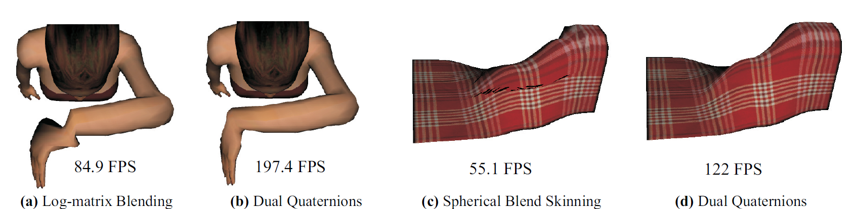

7 Conclusion

In short, dual quaternions are a compact, efficient and elegant technique to represent translations and rotations of physical undeformable objects. This technique allows also interpolation of the information, and achieves nicer results than other techniques with even less memory and better performance.

References

0. Ben Kenwright, A Beginners Guide to Dual-Quaternions, 2011.
1. Ladislav Kavan, Steven Collins, et-al, Dual Quaternions for Rigid Transformation Blending, 2006.
2. Ladislav Kavan, Steven Collins, et-al, Dual Quaternions for Rigid Transformation Blending, 2006.
3. Martin John Baker, Maths - Dual Quaternions, 2015, [Online; accessed 8-December-2015].
4. Wikipedia, Dual quaternion --- Wikipedia, The Free Encyclopedia, 2015, [Online; accessed 8-December-2015].
5. Ben Kenwright, Dual-Quaternions: From Classical Mechanics to Computer Graphics and Beyond, 2012.
6. Martin John Baker, Maths - Dual Numbers, 2015, [Online; accessed 8-December-2015].
7. Wikipedia, Dual number --- Wikipedia, The Free Encyclopedia, 2015, [Online; accessed 8-December-2015].
8. Martin John Baker, Maths - Plücker Coordinates, 2015, [Online; accessed 8-December-2015].

---